학습날짜: 2025.09.03 ~ 2025.09.04
1. Imbalanced Data
1.1. 불균형 데이터
- 불균형 데이터란, 데이터가 한쪽으로 치우쳐 있어서 모델이 고르게 학습하지 못하는 상황을 말함.
- 불균형 데이터를 가진 모델은 데이터가 많은 쪽은 잘 예측하지만, 적은 쪽은 모델 성능이 낮을 것 ⇒ 모델이 편향을 갖게 됨.
# 데이터 불러오기.
# iris 데이터 사용
from sklearn.datasets import load_iris

iris = load_iris()

df = pd.DataFrame(iris["data"], columns=iris["feature_names"])
df["label"] = iris['target']

'''
sepal length (cm)	sepal width (cm)	petal length (cm)	petal width (cm)	label
0	5.1		3.5			1.4			0.2			0
1	4.9		3.0			1.4			0.2			0
2	4.7		3.2			1.3			0.2			0
3	4.6		3.1			1.5			0.2			0
4	5.0		3.6			1.4			0.2			0
'''

# 실습에 사용할 imbalanced data 만들기
# 우선 label 개수 확인
df["label"].value_counts()
'''
	   count
label
0		50
1		50
2		50
'''

# label = 0을 제외한 1,2 를 → 1로 만들기 ()
df['target'] = np.where(df['label'] > 0, 1, 0)
df["target"].value_counts()
'''
		count
target
1		100
0		50
'''
1.2. 분류(Classification)의 경우
✏️ 클래스별 데이터 개수가 고르지 않을 때 발생
예: A 클래스 900개, B 클래스 100개라면 모델은 A만 잘 맞추고 B는 잘 못 맞출 수 있음.
해결 방법
- 부족한 데이터를 추가 확보
- 샘플링(Sampling)
- Under sampling: 가장 적은 데이터 개수를 기준으로 sampling → 유용한 데이터가 사라질 가능성이 높음
- Over sampling: 가장 많은 데이터 개수를 기준으로 적은 데이터는 반복해서 데이터를 추가 sampling → 과적합 발생 가능성
- SMOTE(Synthetic Minority Over-sampling Technique)
- A 보다 B의 데이터가 더 많을 때,
- A 는 over-sampling : KNN 보간법 사용
* 보간법: 알려진 두 점 사이의 값을 이용해 중간 값을 추정하는 방식 - B 는 under-sampling
# SMOTE 라이브러리 불러오기
from imblearn.over_sampling import SMOTE

# SMOTE 실습을 위한 데이터 생성
df_smote = df.copy()
df_smote.dropna(inplace=True)

# X: feature, y: target 분리
X = df_smote.drop(['label', 'target'], axis=1)
y = df_smote['target']

# 계층 추출
x_train, x_test, y_train, y_test = train_test_split(X, y,
                                                    test_size=0.2,
                                                    random_state=11,
                                                    stratify=y)

# 계층 추출 데이터셋 크기 확인
x_train.shape, x_test.shape, y_train.shape, y_test.shape
'''
((119, 4), (30, 4), (119,), (30,))
'''

# SMOTE 객체 생성 (랜덤 시드 고정, k_neighbors=3)
smote = SMOTE(random_state=11, k_neighbors=3)

# 학습 데이터에 SMOTE 적용 → 소수 클래스 샘플을 합성하여 데이터 증강
x_train_over, y_train_over = smote.fit_resample(x_train, y_train)

x_train_over
'''
											count
sepal length (cm)	sepal width (cm)	petal length (cm)	petal width (cm)
5.8			2.700000		5.100000		1.9		2
4.4			2.925186		1.391605		0.2		1
			2.900000		1.400000		0.2		1
			3.000000		1.300000		0.2		1
			3.059990		1.300000		0.2		1
'''

# 계층 추출 vs SMOTE 결과 비교하기
y_train.value_counts(), y_train_over.value_counts()
'''
y_train.value_counts() # 계층 추출
(target
 1    80
 0    39
 Name: count, dtype: int64,

 y_train_over.value_counts() # SMOTE → 클래스 개수 같음
 target
 0    80
 1    80
 Name: count, dtype: int64)
'''- ADASYN (Adaptive Synthetic Sampling)
- SMOTE의 확장판, 그러나 항상 이 방법이 적용되는 것이 아님
- 소수 클래스(minority class) 중에서도 특히 분류가 어려운 샘플(주로 경계 근처)에 더 많은 synthetic data를 생성
- Synthetic Data? 실제로 존재하지 않지만, 통계적·패턴적으로 실제와 유사하게 만들어진 가상의 데이터
# ADASYN 라이브러리 불러오기
from imblearn.over_sampling import ADASYN

# ADASYN 객체 생성
adasyn = ADASYN(random_state=11, n_neighbors=3)

# ADASYN 샘플링
x_train_over, y_train_over = adasyn.fit_resample(x_train, y_train)

'''
---------------------------------------------------------------------------
RuntimeError                              Traceback (most recent call last)
/tmp/ipython-input-2233614973.py in <cell line: 0>()
      1 adasyn = ADASYN(random_state=11, n_neighbors=3)
----> 2 x_train_over, y_train_over = adasyn.fit_resample(x_train, y_train)

3 frames
/usr/local/lib/python3.12/dist-packages/imblearn/over_sampling/_adasyn.py in _fit_resample(self, X, y)
    159             ratio_nn = np.sum(y[nns] != class_sample, axis=1) / n_neighbors
    160             if not np.sum(ratio_nn):
--> 161                 raise RuntimeError(
    162                     "Not any neigbours belong to the majority"
    163                     " class. This case will induce a NaN case"

RuntimeError: Not any neigbours belong to the majority class. This case will induce a NaN case with a division by zero. ADASYN is not suited for this specific dataset. Use SMOTE instead.

이렇게 오류날 떄는 SMOTE 쓰면 됨!!!
'''
1.3. 회귀(regression)의 경우
✏️ 타깃 값이 한쪽으로 몰려 있거나 극단적으로 치우치면, 모델은 편향을 갖게 됨.
1.4. Basic Sampling (실습)
1.4.1. 무작위로 가져오기
# 무작위로 10개 가져오기
rand_samples = df.sample(10)
rand_samples
'''
sepal length (cm)	sepal width (cm)	petal length (cm)	petal width (cm)	label	target
40	5.0		3.5			1.3			0.3			0	0
26	5.0		3.4			1.6			0.4			0	0
58	6.6		2.9			4.6			1.3			1	1
118	7.7		2.6			6.9			2.3			2	1
62	6.0		2.2			4.0			1.0			1	1
120	6.9		3.2			5.7			2.3			2	1
144	6.7		3.3			5.7			2.5			2	1
92	5.8		2.6			4.0			1.2			1	1
64	5.6		2.9			3.6			1.3			1	1
111	6.4		2.7			5.3			1.9			2	1
'''
1.4.2. 계층 추출
# 계층 추출
from sklearn.model_selection import train_test_split

train, test = train_test_split(df, test_size=0.3, random_state=11)
train['target'].value_counts()
'''
	count
target
1	69
0	36
'''

'''
더 정확히 하고 싶다면, 아래와 같이 해야 함.
X_train, X_test, y_train, y_test = train_test_split(
    X, y, test_size=0.3, random_state=11, stratify=y
)
# stratify=y 클래스 비율 유지
'''
1.4.3. 군집 추출(cluster sampling)
# 군집 구간 만들기
num_01 = df['petal length (cm)'].describe()['min']
num_02 = df['petal length (cm)'].describe()['25%']
num_03 = df['petal length (cm)'].describe()['50%']
num_04 = df['petal length (cm)'].describe()['75%']
num_05 = df['petal length (cm)'].describe()['max']

# 군집 생성
df['cluster'] = pd.cut(df['petal length (cm)'],
                       bins = [num_01, num_02, num_03, num_04, num_05], # 구간 나누는 기준 지점이니 사실상 구간은 4개가 나옴
                       labels = ['cluster1', 'cluster2', 'cluster3', 'cluster4'])
df['cluster'].value_counts()

'''
	count
cluster
cluster1	43
cluster3	41
cluster4	34
cluster2	31
'''

# 군집 추출
cond = (df['cluster'] == "cluster1")
df.loc[cond, ]
2.이상값 찾기(Outlier Detection)
2.1. 이상값
이상값(outlier)은 데이터 분포에서 벗어나 모델의 성능을 왜곡할 수 있는 값.
→ 따라서 모델 학습 전 이상치를 탐지하고 적절히 처리하는 과정이 필요함.
# 실습 데이터셋 준비
# 데이터 불러오기
from sklearn.datasets import fetch_openml # 타이타닉 데이터셋

titanic = fetch_openml('titanic', version = 1,as_frame=True)
df = titanic['frame']

'''
참고: df.sex 처럼 점(.) 표기법은 함수 호출과 혼동될 수 있음 → df['sex'] 권장
'''

# 분석에 필요한 컬럼 선택
cols = ["age", "fare"]
df_numeric = df[cols].copy() # shallow copy 방지

# 결측값 확인
df_numeric.isnull().sum()
'''
	0
age	263
fare	1
'''

# 모든 전처리보다 최우적으로 해결해나는 것을 결측값 처리!!!!!!!!!!!!!
# df_numeric['age'].fillna(df_numeric['age'].median(), inplace = True) # 작동은 되나, futureWarning 뜸

# df.method({col: value}, inplace=True) 사용!
# 각 컬럼의 결측값을 중앙값으로 대체
missing_place = {'age': df_numeric['age'].median(),
                 'fare':  df_numeric['fare'].median()}
df_numeric.fillna(missing_place, inplace=True)
2.2. 이상치 처리 절차
- 이상치가 포함된 데이터 행(row)의 index를 찾음
- 해당 index를 제외한 데이터 확보
2.3. 이상치 탐지 방법
- Boxplot 응용
- Tukey 방식: outlier boundary = 1.5 × IQR
- Carling 방식: outlier boundary = 2.3 × IQR
# 이상치 탐지 함수 생성(IQR 방식, Tukey 기준)
def outlier_detection(data, column):
  IQR = data[column].quantile(0.75) - data[column].quantile(0.25)
  lb = data[column].quantile(0.25) - (1.5 * IQR)
  ub = data[column].quantile(0.75) + (1.5 * IQR)

  cond = (data[column] < lb) | (data[column] > ub)
  outlier_value = data.loc[cond,]

  return outlier_value

# fare 컬럼 이상치 탐지 및 확인
outlier_fare = outlier_detection(df_numeric, 'fare')
outlier_fare.shape, df_numeric.shape
'''
((171, 2), (1309, 2))
'''

# 이상치 제거(fare 기준)
df_numeric[~df_numeric['fare'].isin(outlier_fare)]
- ESD (Extreme Studentized Deviate)
- 데이터가 정규성을 가진다는 가정하에서 사용
- 평균 ± 2σ (또는 3σ) 밖에 있는 값을 이상치로 지정
# 평균과 분산 먼저 확인
df_numeric['fare'].mean(), df_numeric['fare'].std()
'''
(np.float64(33.281085637891515), 51.74149976752598)
'''

# 이상치 탐지 함수 생성(ESD 방식)
def esd_detection(data, column, num):
  m = data[column].mean()
  s = data[column].std()

  ub = m + (s * num)
  lb = m - (s * num)

  cond = (data[column] < lb) | (data[column] > ub)
  outlier_value = data.loc[cond,]

  return outlier_value

# fare 컬럼 이상치 탐지 및 확인
outlier_fare = esd_detection(df_numeric, 'fare', 2)
outlier_fare.shape, df_numeric.shape

# 이상치 제거(fare 기준)
df_numeric.drop(index = outlier_fare.index)
- LOF (Local Outlier Factor)
- "지역적(local)" 밀집도를 기준으로 이상치 탐지
- 여러 차원을 동시에 고려할 수 있어 다차원 이상치 탐지에 효과적
- 정상 데이터는 이웃과 유사한 밀도를 가지지만, 이상치는 낮은 밀도를 가질 것으로 예상
- LOF < 1: 밀도가 높은 분포
- LOF = 1: 이웃과 유사한 분포
- LOF > 1: 밀도가 낮은 분포 → 이상치 정도가 클수록 값이 큼
- ⚠ LOF는 거리 기반이므로 스케일링 필수
# 거리를 다루는 모형들을 무조건 스케일링해야 함!
from sklearn.preprocessing import StandardScaler # 스케일링 라이브러리

# 스케일링 객체 생성
scaler = StandardScaler()

# 스케일링 (평균 0, 분산 1로 변환)
X_scaled = scaler.fit_transform(df_numeric)

# LOF(Local Outlier Factor) 라이브러리 불러오기
from sklearn.neighbors import LocalOutlierFactor

# LOF 객체 생성 (이웃=20명, 이상치 비율 5%로 설정)
lof = LocalOutlierFactor(n_neighbors=20, contamination=0.05)

# LOF 적용 (-1: 이상치, 1: 정상치)
y_pred = lof.fit_predict(X_scaled)

# lof지수 확인
lof_score = -lof.negative_outlier_factor_ # 밀도 값
lof_score
'''
array([ 0.97304705,  2.39372781,  2.31880549, ...,  1.02368054,
       52.50738275, 73.77181185])
'''

# 결과 정리: 원본 데이터 + LOF 점수 + 이상치 여부
df_result = df_numeric.copy()
df_result['LOF_Score'] = lof_score
df_result['Anomaly'] = y_pred

# 이상치 제거
cond = (df_result['Anomaly'] == -1)
outlier_index = df_result.loc[cond, ].index
df_result.drop(index = outlier_index)
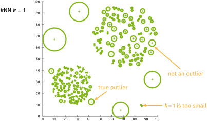
- KNN Model을 이용한 Anormaly Detection(KNN 기반 이상치 탐지)
# 실습 데이터 만들기 - iris 데이터 사용
from sklearn.datasets import load_iris

data = load_iris()
df = pd.DataFrame(data['data'], columns = data['feature_names'])
df['species'] = data['target']

# sepal length, sepal width만 선택 (단위 동일 → 스케일링 생략)
cols = ['sepal length (cm)', 'sepal width (cm)']
df = df.loc[:, cols]
df.columns = ['sepal length', 'sepal width']

# KNN 라이브러리 불러오기
from sklearn.neighbors import KNeighborsClassifier

# KNN 모델 학습 (이웃 개수 = 3)
nbrs = KNeighborsClassifier(n_neighbors = 3)
nbrs.fit(x, y)

# 각 샘플별 KNN 거리 계산
# distances: 각 데이터 포인트와 이웃 간의 거리(자기자신, 이웃1, 이웃2)
# indexed: 이웃 데이터의 인덱스
distances, indexed = nbrs.kneighbors(x)

# 이상치 판단 기준(rule) 설정
# thr > 0.15(평균거리) → 이상치판단
outlier_index = np.where(distances.mean(axis=1) > 0.15)

# 참고:
# np.where(조건1, true 값, false 값)
# np.where(조건) : 해당조건에 대한 array의 index값

# 이상치 값 확인
outlier_val = df.loc[outlier_index]
outlier_val.head(3)
'''
sepal length	sepal width
14	5.8	4.0
15	5.7	4.4
18	5.7	3.8
'''
3. 결측치(NaN) 처리_심화2
이전에 다룬 단순 결측치 처리 방법 외에, 머신러닝에서 활용할 수 있는 대체 기법(imputation) 을 학습
여기서는 단순 삭제가 아닌, 데이터를 적절히 보완하는 방식에 초점을 맞춤!
# 실습 데이터 가져오기 - 타이타닉 데이터셋 사용
from sklearn.datasets import fetch_openml

titanic = fetch_openml('titanic', version = 1,as_frame=True)
df = titanic['frame']
3.1. KNN Imputer
- 가까운 이웃들의 값(거리 기준)을 활용해 결측치를 대체
# 분석 대상: age, fare 컬럼만 추출 (결측치 제거)
cols = ["age", "fare"]
df_numeric = df[cols].dropna()

# 스케일링 (거리 기반 알고리즘 → 반드시 필요)
from sklearn.preprocessing import StandardScaler
scaler = StandardScaler()
X_scaled = scaler.fit_transform(df_numeric)

# 이상치 탐지 → NaN으로 처리 → KNN Imputer로 값채우기
# LOF(Local Outlier Factor)로 이상치 탐색
lof = LocalOutlierFactor(n_neighbors=20, contamination=0.05) # 이상치 비율
y_pred = lof.fit_predict(X_scaled) # -1: 이상치, 1: 정상치

# 이상치 여부를 데이터프레임에 추가
df_numeric["Anormaly"] = y_pred

# 이상치를 NaN으로 처리
cond = (df_numeric["Anormaly"] == -1)
df_numeric.loc[cond, cols] = np.nan

# KNN Imputer로 결측치 대체
from sklearn.impute import KNNImputer # KNN Imputer 라이브러리 불러오기

# 이웃 5개를 기준으로 imputer 객체 생성
imputer = KNNImputer(n_neighbors = 5)

# NaN → 이웃값으로 보완 (결과는 numpy 배열로 반환됨)
imput_values = imputer.fit_transform(df_numeric[cols])
imput_values
'''
array([[ 29.        , 211.3375    ],
       [ 30.06829637,  34.81990474],
       [ 30.06829637,  34.81990474],
       ...,
       [ 26.5       ,   7.225     ],
       [ 27.        ,   7.225     ],
       [ 29.        ,   7.875     ]])
'''
3.2. Regression Imputer
- 변수 간 상관관계가 있는 경우, 회귀 모델로 결측치를 예측하여 대체
- 전제조건 필요
- 예: age 값을 예측할 때, fare와 상관성이 있다면 fare를 기반으로 age의 결측값을 보완
# 분석 대상: age, fare 컬럼만 추출
cols = ["age", "fare"]
df_numeric = df[cols].copy()

# fare 결측치는 중앙값으로 간단히 대체
df_numeric['fare'] = df_numeric['fare'].fillna(df_numeric['fare'].median())

# age 결측치 처리 준비
train = df_numeric.dropna(subset = ['age']) # 결측값이 없는 age
cond = df_numeric['age'].isna()
test = df_numeric.loc[cond] # 결측값이 있는 age

# 결측측 없는 데이터로 학습용 데이터 만들기 (X=요금, y=나이)
col = ['fare']
x_train = train[col]
y_train = train['age']

# 선형회귀 모델 학습 (fare → age 예측)
from sklearn.linear_model import LinearRegression # 선형회귀모델 라이브러리
reg = LinearRegression()
reg.fit(x_train, y_train)

# 결측치가 있는 age 데이터 예측
col = ['fare']
x_test = test[col] # DataFrame 형태 유지 (2D)
y_age_pred = reg.predict(x_test)

# 참고: test['fare'] → series(1d) / test[['fare']] → df(2d)

# age 결측치 대체
df_numeric.loc[cond, 'age'] = y_age_pred
'LG U+ Why Not SW Camp 8기 > 학습 로그' 카테고리의 다른 글
| 공부 일지 #33 | 머신러닝 : 규제와 분류(로지스틱, 성능지표) (0) | 2025.09.07 |
|---|---|
| 공부 일지 #32 | 머신러닝: 회귀 (0) | 2025.09.07 |
| 공부 일지 #30 | 머신러닝 전처리: 과대적합·과소적합, 인코딩, 스케일링 (0) | 2025.09.07 |
| 공부 일지 #29 | 머신러닝 경험해보기: KNN 알고리즘 (0) | 2025.09.05 |
| 공부 일지 #28 | 머신러닝 첫걸음: 개념, 유형, 흐름 (1) | 2025.09.03 |