학습날짜: 2025.09.08
1. 분류 모델의 성능 측정: ROC Curve와 AUC
1.1. 기존 성능 지표와 한계
- 정확도, 정밀도, 재현율, F1-score → 이론적 지표 성격 강함
- 데이터셋 특성 따라 신뢰할 수 있는 지표가 다름
- 기존 지표는 TP 중심이라 FP/FN은 부분적으로만 반영됨 ∴ 모델 전반 성능 설명엔 부족, 이론적 지표라 불림
- 실무에서는 ROC, AUC 많이 씀
1.2. ROC Curve 개념
- ROC (Receiver Operation Characteristic): 모든 분류 임계값에서 모델 성능 보여주는 그래프
- 임계값(Threshold)
- 0 → 거의 다 Positive로 분류 → 좌표 (1,1)
- 1 → 거의 다 Negative로 분류 → 좌표 (0,0)
- 0~1 값 변화에 따라 FPR, TPR 값이 변하며 ROC 커브가 그려지고, 면적이 결정됨
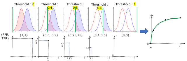
- x축 = FPR (False Positive Rate, 허위양성비율). 값 클수록 성능 나쁨
- y축 = TPR (True Positive Rate = Recall). 값 클수록 성능 좋음
- 따라서, 좋은 모델은 y축으로 치우친(왼쪽 위로 볼록한) 그래프를 가짐.
# --- 이전 과정 ---
# 1. 데이터 불러오기 및 전처리
# 2. y값 생성 (count >= 500 → 1, 그 외 → 0)
# 3. 스케일링 및 train/test 분리
# 4. 로지스틱 회귀 모델 학습 및 예측
# 5. classification_report로 기본 성능 지표 확인
# ----------------

# ROC 커브 그리기 위한 확률 예측값 생성
predict_proba = clf.predict_proba(x_test)  # 클래스별 확률 반환 | [0일 확률, 1일 확률]

# 양성 클래스(1)에 대한 확률값만 사용
proba_class1 = predict_proba[:, 1]

# ROC 커브 계산
from sklearn.metrics import roc_curve

fprs, tprs, thresholds = roc_curve(y_test, proba_class1)

# ROC 커브 시각화
import matplotlib.pyplot as plt

def roc_curve_plot(y_test, predict_proba_p):
    fprs, tprs, thresholds = roc_curve(y_test, predict_proba_p)
    plt.plot(fprs, tprs, label="ROC")
    plt.plot([0,1], [0,1], label="random")  # 기준선
    plt.xlabel("FPR")
    plt.ylabel("TPR")

    plt.show()

roc_curve_plot(y_test, proba_class1)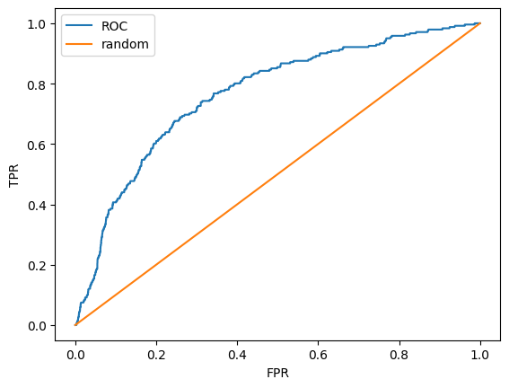
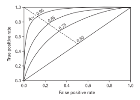
1.3. AUC (Area Under Curve)
- ROC Curve 아래 면적을 뜻하며, 커질수록 성능 좋음
- 보통 0.9 이상이면 우수한 모델로 간주, 0.5 이하는 무의미(랜덤 분류 수준)
- AUC가 클수록 TPR 증가 시 FPR의 증가가 억제됨
- 기업에서는 특히 FPR이 중요 → 가짜 불량률이 낮아야 하기 때문.
- Recall(=TPR)은 여전히 중요한 이론적 지표이므로, 결국 TPR은 높이고 FPR은 억제하는 튜닝이 필요
- 보조 지표로 Precision-Recall Curve도 활용 가능 (AUC의 좌우 반전 형태)

# AUC 점수 계산
from sklearn.metrics import roc_auc_score

auc_score = roc_auc_score(y_test, proba_class1)

print("AUC Score:", auc_score)
'''
np.float64(0.7653743012928227)
.90 을 넘지 않기 때문에, 좋은 모델 아님!
'''
2. Decision Tree 모델
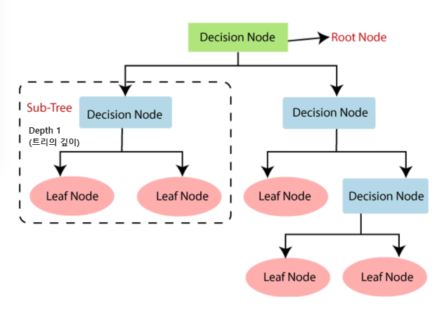
- Decision Tree = Mother 모델이라 불림. 회귀와 분류 둘 다 가능하지만 보통 분류에 많이 씀.
- 트리 구조로 학습 → Root Node, Decision Node, Leaf Node, Depth 개념 중요
- Depth 깊을수록 학습량 많아지지만, 너무 깊으면 과적합(overfitting)됨
- y값이 섞여 있으면 불순도(impurity) 높음. 학습은 불순도를 낮추는 방향으로 진행됨
- 다른 모델과 다르게 시각화 가능
2.1. 불순도와 엔트로피 (Entropy)
- y값 섞이면 불순도 높음, 한쪽으로 몰리면 낮음
- 학습 목표 = 불순도 줄이는 방향
- 불순도 지표
- Entropy: H(p) = – Σ pᵢ log₂(pᵢ)
- Gini 불순도: Gini = 1 – Σ pᵢ²
- Variance: 회귀 트리에서 사용
- 엔트로피 특징
- all(+) or all(-) → Entropy = 0 (순수)
- 반반 섞이면 Entropy 최대 (역U 형태)
2.2. 정보이득 (Information Gain, IG)
- 정보이득 = 부모 노드 불순도 – 가중평균(자식 노드 불순도)
- 분할했을 때 불순도가 얼마나 줄었는지 나타내는 지표
- 값이 클수록 좋은 분할, IG 큰 변수가 Decision Node로 선택됨
2.3. 질문(분할 기준) 선택 원리
- Decision Tree 학습 핵심은 좋은 질문(조건)을 고르는 것
- 기준
- 노드 내 동질성 ↑
- 순도 ↑
- 불순도 ↓ (핵심)
- 정보이득(IG) ↑
2.4. 학습 알고리즘
- 기본 패턴
- dataset → IG 크게 만드는 방향으로 분할 → 반복
- y값이 섞여 있지 않음 = 불순도 0 → 학습 종료
- 문제점
- impurity = 0까지 가면 과적합 발생
- 이를 막기 위해 가지치기(pruning) 필요
2.4.1. Pruning (가지치기) 기법
- Early Stopping (사전 가지치기, Pre-pruning)
- 학습 도중 조건을 걸어 트리 성장을 미리 멈추는 방식
- 방법
- Depth 제한 → 특정 깊이 이상 학습 중단
- Leaf Node 조건 → ex) 노드 샘플 수 일정 기준 미만이면 stop
- Min Samples per Split → 분할 최소 샘플 수 조건
- Min IG, Min Impurity Decrease 등 하이퍼파라미터 활용
- Post-pruning (사후 가지치기)
- 트리를 끝까지 만든 뒤 불필요한 가지 제거하는 방식
- Early Stopping과 달리 사후에 가지를 줄이는 접근
2.5. 분류 vs 회귀
- Classification Tree
- 중요한 변수 기준으로 Decision Node 생성
- y값 불순도 줄이는 방향으로 분할
- Regression Tree
- 영역을 나누어 연속형 값 예측
- 불순도 대신 분산(Variance) 줄이는 방향으로 학습
2.6. 특징
- 장점
- 시각화 가능 → 모델 해석 용이
- 비모수적 방법 → 데이터 분포 가정 필요 없음
- 전처리 영향 적음 (Scaling, One-hot 등 크게 중요치 않음)
- Feature Selection 자동 수행
- 단점
- 과적합에 취약
- 데이터 불균형 문제 발생 가능
- 변수 많으면 학습 속도 느려짐
- 다른 모델 대비 예측 정확도 낮은 편
- 학습 시간·공간 복잡도 높음
2.7. 실습
# --- 데이터 준비 ---
from sklearn.datasets import load_breast_cancer   # 유방암 데이터셋 로드
import pandas as pd                               # 데이터프레임 변환
from sklearn.model_selection import train_test_split  # train/test 분리
from sklearn.metrics import classification_report     # 성능 평가 지표

# --- 모델 학습 & 시각화 관련 ---
from sklearn import tree                          # Decision Tree 모델
from sklearn.tree import export_graphviz          # 트리 시각화용 DOT 파일 생성
import pydotplus                                  # DOT 데이터를 그래프로 변환
from IPython.display import Image                 # Jupyter에서 이미지 출력

# 유방암 데이터셋 로드
cancer = load_breast_cancer()

# 데이터프레임으로 변환
df = pd.DataFrame(cancer['data'], columns=cancer['feature_names'])
df['label'] = cancer['target']
df.head()

# train/test 분리
x_train, x_test, y_train, y_test = train_test_split(cancer['data'],
                                                    cancer['target'],
                                                    test_size=0.3,
                                                    random_state=12)

# --- 기본 모델 학습 ---
dt = tree.DecisionTreeClassifier(random_state=12)   # Decision Tree 객체 생성
dt.fit(x_train, y_train)                            # 모델 학습

print(f"Depth of tree: {dt.get_depth()}")           # 트리 깊이 확인
print(f"Number of leaves: {dt.get_n_leaves()}")     # 리프 노드 개수 확인
'''
Depth of tree: 6
Number of leaves: 13
'''

# 예측 및 성능 평가
y_pred = dt.predict(x_test)
print(classification_report(y_test, y_pred))
'''
              precision    recall  f1-score   support

           0       0.92      0.84      0.88        64
           1       0.91      0.95      0.93       107

    accuracy                           0.91       171
   macro avg       0.91      0.90      0.90       171
weighted avg       0.91      0.91      0.91       171
'''

# --- 트리 시각화 ---
dot_data = export_graphviz(dt,
                           feature_names=cancer['feature_names'], # 변수명
                           class_names=cancer['target_names'],   # 클래스명
                           filled=True,                          # 색상
                           rounded=True)                         # 둥근 모서리

graph = pydotplus.graph_from_dot_data(dot_data)     # DOT 데이터를 그래프로 변환
Image(graph.create_png())                           # 이미지 출력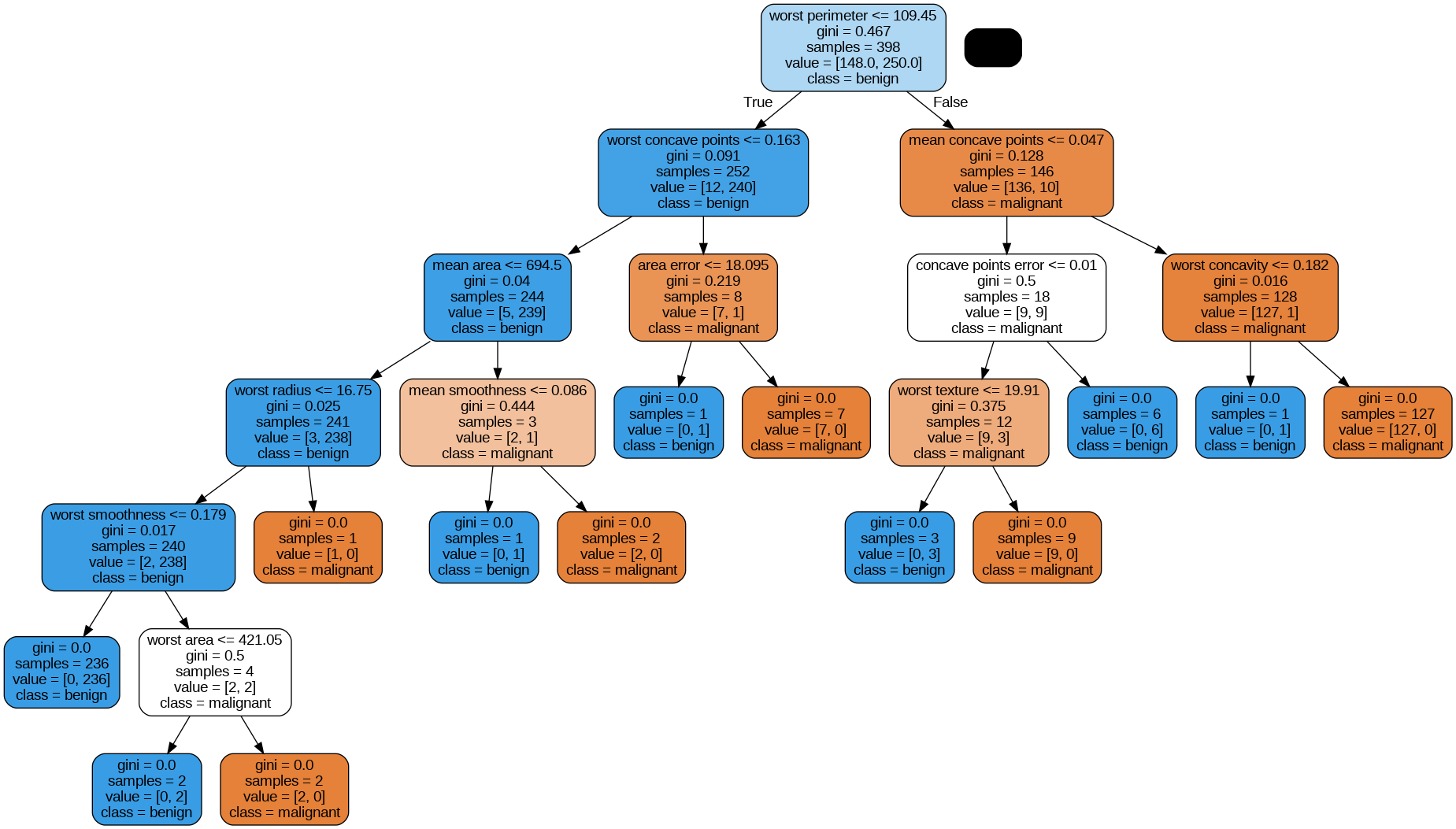
# --- max_depth 변화에 따른 성능 비교 ---
depths = [1, 2, 3, 4, 5]
outputs = []

for depth in depths:
    model = tree.DecisionTreeClassifier(max_depth=depth, random_state=12)
    model.fit(x_train, y_train)
    y_pred = model.predict(x_test)
    outputs.append(classification_report(y_test, y_pred))

# depth별 성능 출력
for index, data in zip(depths, outputs):
    print(f"depth: {index}")
    print(data)  # support = 각 클래스의 실제 샘플 개수
'''
depth: 1
              precision    recall  f1-score   support

           0       0.83      0.77      0.80        64
           1       0.87      0.91      0.89       107

    accuracy                           0.85       171
   macro avg       0.85      0.84      0.84       171
weighted avg       0.85      0.85      0.85       171

depth: 2
              precision    recall  f1-score   support

           0       0.83      0.86      0.85        64
           1       0.91      0.90      0.91       107

    accuracy                           0.88       171
   macro avg       0.87      0.88      0.88       171
weighted avg       0.88      0.88      0.88       171

depth: 3
              precision    recall  f1-score   support

           0       0.90      0.86      0.88        64
           1       0.92      0.94      0.93       107

    accuracy                           0.91       171
   macro avg       0.91      0.90      0.91       171
weighted avg       0.91      0.91      0.91       171

depth: 4
              precision    recall  f1-score   support

           0       0.90      0.86      0.88        64
           1       0.92      0.94      0.93       107

    accuracy                           0.91       171
   macro avg       0.91      0.90      0.91       171
weighted avg       0.91      0.91      0.91       171

depth: 5
              precision    recall  f1-score   support

           0       0.89      0.86      0.87        64
           1       0.92      0.93      0.93       107

    accuracy                           0.91       171
   macro avg       0.90      0.90      0.90       171
weighted avg       0.91      0.91      0.91       171
'''

# --- 최적 depth = 3 선택 ---
best_dt = tree.DecisionTreeClassifier(max_depth=3, random_state=12)
best_dt.fit(x_train, y_train)
y_pred = best_dt.predict(x_test)

# 최적 depth 트리 시각화
dot_data = export_graphviz(best_dt,
                           feature_names=cancer['feature_names'],
                           class_names=cancer['target_names'],
                           filled=True,
                           rounded=True)

graph = pydotplus.graph_from_dot_data(dot_data)
Image(graph.create_png())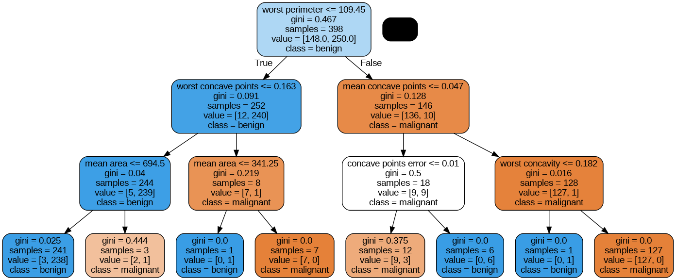
'LG U+ Why Not SW Camp 8기 > 학습 로그' 카테고리의 다른 글
| 공부 일지 #36 | 머신러닝: 나이브베이즈와 군집분석(비지도) (0) | 2025.09.14 |
|---|---|
| 공부 일지 #35 | 머신러닝: 앙상블과 RandomForest, 교차검증 (0) | 2025.09.14 |
| 공부 일지 #33 | 머신러닝 : 규제와 분류(로지스틱, 성능지표) (0) | 2025.09.07 |
| 공부 일지 #32 | 머신러닝: 회귀 (0) | 2025.09.07 |
| 공부 일지 #31 | 머신러닝 전처리: 불균형 데이터·이상치·결측치 처리 (0) | 2025.09.07 |