학습 날짜: 2025.08.19
오늘은 Google Colab 환경에서 Python과 Matplotlib, pandas 라이브러리를 활용하여 여러 가지 시각화 연습을 해보았다.
배운 내용 전체를 다 담기보다는, 각 그래프 유형별로 대표적인 코드 한두 개씩만 기록하여 정리해 두고자 한다.
Matplotlib
Linplot(선 그래프)
x: 연속형 ~ y: 연속형
plt.figure(figsize=(10, 5)) # 도화지 생성

plt.plot(x, .5 + x, "--") # "--": 점선으로 표현
plt.plot(x, 1 + 2 * x, "r^") # "bo": 파란색 굵은 원 점선으로 표현, "b*": 파란색 * 점선으로 표현
plt.plot(x, 1 + 6 * x, "g") # "g" : 초록색 실선

plt.show() # 그래프 출력
Histogram(히스토그램)
x: 연속형 ~ y: 빈도(도수)
x = df["humidity"]
plt.figure(figsize=(10, 5))
plt.hist(x, bins = 50)
plt.show()
Box plot(상자 그림)
x: 범주형 ~ y: 연속형
# 다변량 box plot
cond_f = ((df["Gender"] == "f") | (df["Gender"] == "F")) & (df["Distance"] < 5000)
cond_m = ((df["Gender"] == "m") | (df["Gender"] == "M")) & (df["Distance"] < 5000)

plt.figure(figsize=(10, 5))

plt.boxplot(
    [df.loc[cond_f, "Distance"], df.loc[cond_m, "Distance"]],
    labels=["Female", "Male"]
)
plt.title("Distance (<5000) by Gender")
plt.xlabel("Gender")
plt.ylabel("Distance")

plt.show()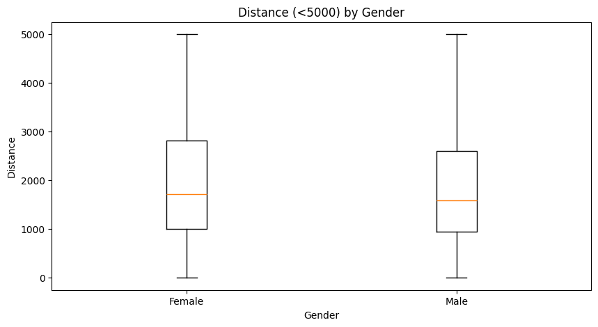
Bar chart(막대 그래프)
x: 범주형 ~ y: 연속형
language = ["Python", "R", "SQL", "Java"]
votes_20 = [91, 82, 78, 75]
votes_19 = [88, 92, 81, 87]

x1 = np.linspace(1, 10, num=4) # bar 자리 잡기
x2 = x1 + 0.8  # bar2 간격띄우기

fig = plt.figure()
ax = fig.subplots(1,1) #nrow =1, ncol=1

ax.bar(x1, votes_20)
ax.bar(x2, votes_19)

middle_x = [(a + b)/2 for (a,b) in zip(x1, x2)]
ax.set_xticks(middle_x)
ax.set_xticklabels(language)

plt.legend(['y2020', 'y2019'])
plt.show()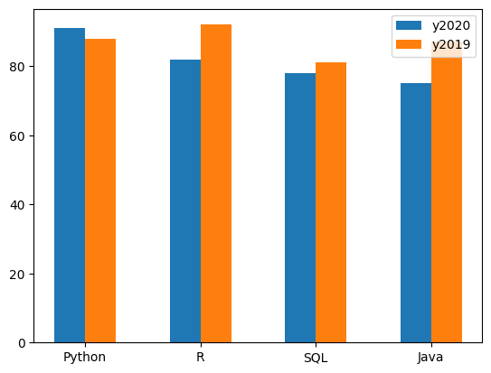
Stacked bar chart(누적 막대 그래프)
x = ["a", "b", "c", "d"]
y1 = [1, 2, 3, 4]
y2 = [3, 4, 5, 6]

plt.figure(figsize=(8, 5))
plt.bar(x, y1)
plt.bar(x, y2, bottom = y1)

plt.show()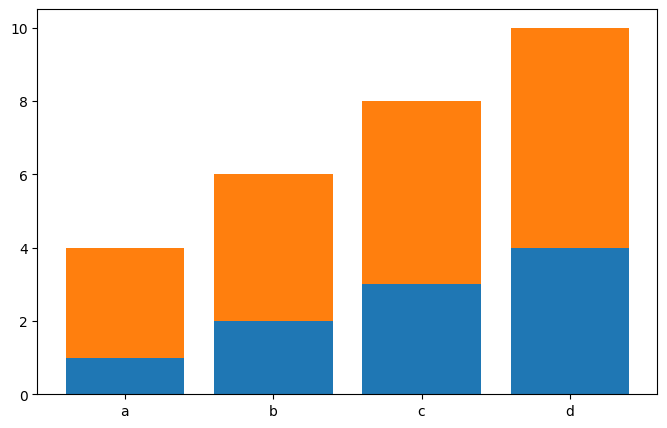
Pie chart(원 차트)
x: 범주형 ~ 비율(%)
colors = [ 'yellowgreen','lightskyblue', 'lightcoral', 'blue', 'coral']

sizes = df["Gender"].value_counts()
labels = df["Gender"].unique()
explode = (0.05, 0, 0) # 파이끼리의 간격 조정

plt.pie(sizes, labels = labels, colors = colors, explode = explode, autopct='%1.1f%%')
# 1.1f% = '정수.소수점 자리 float%'로 표현

plt.show()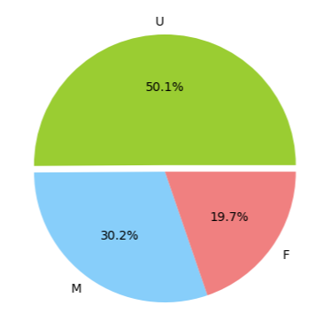
Scatter plot(산점도)
x: 연속형 ~ y: 연속형
plt.figure(figsize = (8,5))

plt.scatter(x = "Carbon_amount", y = "Momentum", data = df) # 어떠한 패턴이 있는듯...?
plt.show()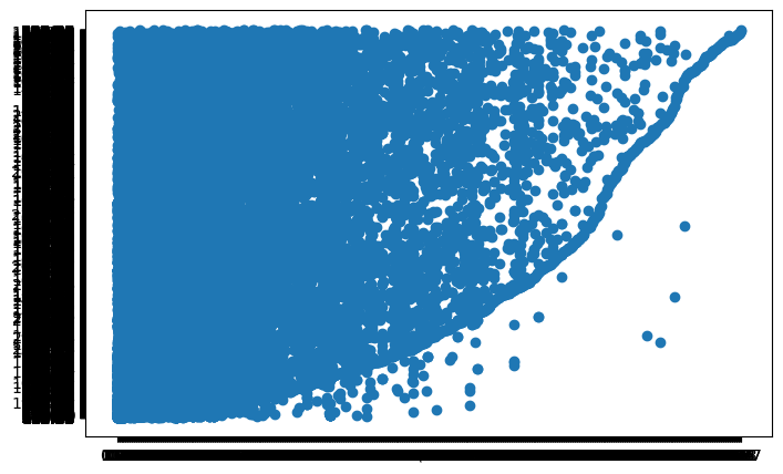
EDA(탐색적데이터분석); 시 그래프 활용
def graph_display(col, y_value, target_df):
  plt.figure(figsize=(8,5))

  plt.scatter(x=col, y=y_value, data=target_df)
  plt.show()

target_df = df.select_dtypes(include="int")
target_df.head()

cols = target_df.columns[:-2]
y_value = "Duration"
for col in cols:
  graph_display(col, y_value, target_df)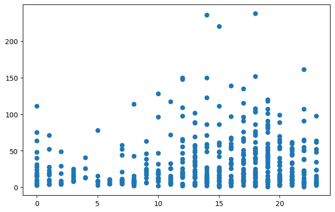
Pandas
Linplot(선 그래프)
# 읽어들인 시계열데이터를 line chart로 표현해보세요.
df_csv.plot(kind="line",
            x="Month", y="MW",
            title = "MW ~ Month",
            ylabel="MW",
            figsize=(12, 5))
plt.show()
Histogram(히스토그램)
df_excel["Momentum"].plot(kind="hist",
                          figsize=(8, 5),
                          title = "Histogram",
                          xlabel="Momentum")
plt.show()
Box plot(상자 그림)
# 'Momentum' 컬럼의 정보를 'Gender'별로 구분해서 boxplot을 그리고 해석해보세요.
df_excel.boxplot(column='Momentum', by = 'Gender')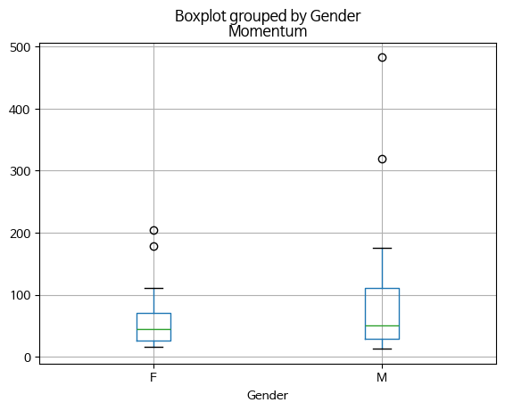
Bar chart(막대 그래프)
(option) stacked = True 사용시, 누적 막대 그래프로 표현됨
# Creating bar plot using more than two variables from the crosstab
# 판다스의 crosstab을 이용해서 'Gender'별로 그루핑하고,
# 'Membership_type', 'Age_Group'에 대한 pair counting정보를 bar chart로 보여주세요.

pair_cols = [df_excel['Age_Group'], df_excel['Membership_type']]
data = pd.crosstab(df_excel['Gender'], pair_cols)

data.plot(kind = 'bar', rot = 0, ylabel="Frequency")
Pie chart(원 차트)
#위에서 구성된 빈도교차표를 이용해서 '일일권', '정기권'에 대한 파이차트를 그려보세요.

data = pd.crosstab(df_excel['Age_Group'], df_excel['Membership_type'])
data.plot(kind="pie", subplots=True, figsize=(12,5))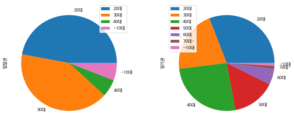
Scatter plot(산점도)
# Scatter plot of two columns
# dataframe을 이용해서 x축에 'Distance'컬럼, y축에 'Momentum' 컬럼의 데이터를 설정해서 산점도를 그려보세요.

df_excel.plot.scatter(x = 'Distance', y = 'Momentum')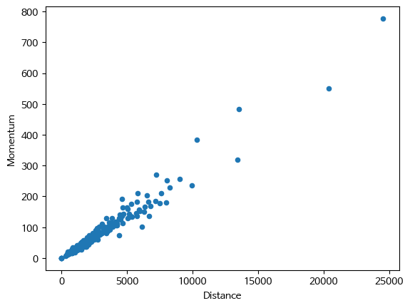
Heatmap(히트맵)
seaborn 라이브러리 사용
- pivot_table로 변환이 필수임!
# pivot_table 변환 필수
# 관심값: 탑승객 수, month으로 grouping, x축: year
df_pivot = pd.pivot_table(df, index="month", values="passengers", columns="year")
df_pivot.head()

sns.heatmap(df_pivot, annot=True, fmt='.0f')
plt.title('passengers ~ month + year')
plt.figure(figsize= (10,10))
plt.show()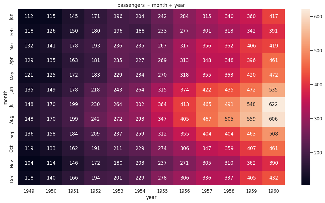
'LG U+ Why Not SW Camp 8기 > 학습 로그' 카테고리의 다른 글
| 공부 일지 #26 | 통계 및 실습: 상관, 회귀 (4) | 2025.08.26 |
|---|---|
| 공부 일지 #25 | 추론과 검정 정리: 추정, 가설검정, t-test, ANOVA, 카이제곱 (4) | 2025.08.24 |
| 공부 일지 #23 | Python Pandas 데이터 분석 기초 함수 (0) | 2025.08.19 |
| 공부 일지 #22 | 데이터 분석 기초 정리2: 자유도, 분포, 기초통계량 (3) | 2025.08.18 |
| 공부 일지 #21 | Python Pandas 기본 문법 정리: 데이터 전처리 기초 (8) | 2025.08.14 |